Gaussian Mixture - 2D
Description:
Optimization (max)
Multimodal (yes)
This function provides a 2D Gaussian mixture model.
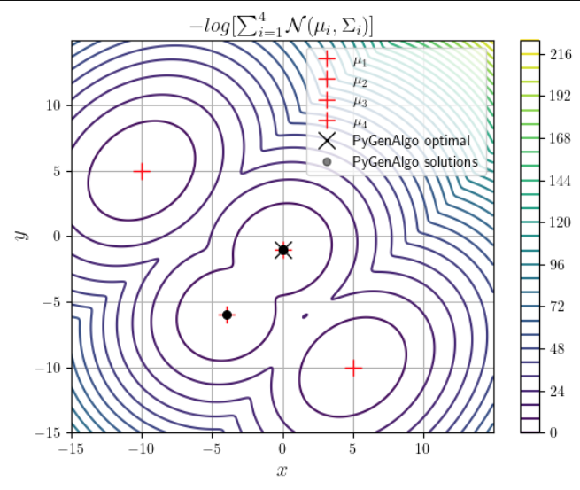
The equations are given by the Multivariate Normal Distribution, with four modes (2 global and 2 local):
\[f(x) = \sum_{i=1}^{4} \mathcal{N}(\mu_i, \Sigma_i)\]with mean vectors:
\[ \begin{align}\begin{aligned}\mu_1 = [-0.0, -1.0]\\\mu_2 = [-4.0, -6.0]\\\mu_3 = [-5.0, +1.0]\\\mu_4 = [5.0, -10.0]\end{aligned}\end{align} \]and covariances:
\[ \begin{align}\begin{aligned}\Sigma_1 = [ [ 1.0, 0.1 ], [ 0.1, 1.0 ] ]\\\Sigma_2 = [ [ 1.0, 0.1 ], [ 0.1, 1.0 ] ]\\\Sigma_3 = [ [ 1.2, 0.3 ], [ 0.3, 1.2 ] ]\\\Sigma_4 = [ [ 1.2, 0.3 ], [ 0.3, 1.2 ] ]\end{aligned}\end{align} \]
Step 1: Import python libraries and PyGenAlgo classes
import numpy as np
from matplotlib import pyplot as plt
from scipy.stats import multivariate_normal

# Enable LaTex in plotting.
plt.rcParams["text.usetex"] = True

# Import main classes.
from pygenalgo.genome.gene import Gene
from pygenalgo.genome.chromosome import Chromosome
from pygenalgo.utils.utilities import cost_function
from pygenalgo.engines.standard_ga import StandardGA

# Import Selection Operator(s).
from pygenalgo.operators.selection.neighborhood_selector import NeighborhoodSelector

# Import Crossover Operator(s).
from pygenalgo.operators.crossover.blend_crossover import BlendCrossover

# Import Mutation Operator(s).
from pygenalgo.operators.mutation.gaussian_mutator import GaussianMutator
Step 2: Define the objective function
# Setup the 2D Gaussian functions.
# NOTE: Because of their covariance setup, the first two (mvn_1 and mvn_2)
# will have higher modes then the other two. So the maximum will be in one
# of these two modes.

# Each one with different mean and covariance matrix.
mvn_1 = multivariate_normal([-0.0, -1.0], [[1.0, 0.1], [0.1, 1.0]])

mvn_2 = multivariate_normal([-4.0, -6.0], [[1.0, 0.1], [0.1, 1.0]])

mvn_3 = multivariate_normal([-10.0, 5.0], [[1.2, 0.3], [0.3, 1.2]])

mvn_4 = multivariate_normal([5.0, -10.0], [[1.2, 0.3], [0.3, 1.2]])

# Define the negative log of the pdfs.
def negative_log_pdfx(x: np.ndarray) -> float:
    return -np.log(mvn_1.pdf(x) + mvn_2.pdf(x) + mvn_3.pdf(x) + mvn_4.pdf(x))
# _end_def_

# Multimodal cost function.
@cost_function(minimize=True)
def fun_test2D(individual: Chromosome) -> float:

    # Extract the x, y values.
    x, y = individual.values()

    # Compute the final value.
    f_value = negative_log_pdfx([x, y])

    # Return the solution.
    return f_value.item()
Step 3: Set the GA parameters
# Set a seed for reproducible initial population.
SEED = 1821

# Random number generator.
rng = np.random.default_rng(SEED)

# Random function that enforce the boundaries in x/y.
boundary_xy = lambda: rng.uniform(-15.0, 15.0)

# Define the number of chromosomes.
n_pop, n_dim = 50, 2

# Draw random samples for the initial points.
xy_init = rng.uniform(-15.0, 15.0, size=(n_pop, n_dim))

# Initial population.
population = [Chromosome([Gene(xy_init[i, 0], boundary_xy),
                          Gene(xy_init[i, 1], boundary_xy)], np.nan, True)
              for i in range(n_pop)]

# Create the StandardGA object that will carry on the optimization.
test_GA = StandardGA(initial_pop=population,
                     fit_func=fun_test2D,
                     select_op=NeighborhoodSelector(),
                     mutate_op=GaussianMutator(lower_val=-15.0,
                                               upper_val=+15.0),
                     crossx_op=BlendCrossover(lower_val=-15.0,
                                              upper_val=+15.0))
Step 4: Run the optimization
test_GA(epochs=500, elitism=False, shuffle=False, verbose=False)
Step 5: Extract the data for analysis and plotting
# Extract the data values as 'x' and 'y', for parsimony.
x_opt, y_opt = test_GA.best_chromosome().values()

# Compute the final objective functions.
f_opt = negative_log_pdfx([x_opt, y_opt])

# Print the results.
print(f"x={x_opt:.5f}, y={y_opt:.5f}", end='\n\n')
print(f"f_opt(x, y) = {f_opt:.5f}")
Step 6: Visualize the solutions
# Store the additional solutions.
best_n = []

for p in test_GA.best_n(n=n_pop//2):
    best_n.append(p.values())

best_n = np.array(best_n)

# Prepare the plot of the real density.
x, y = np.mgrid[-15:15:0.01, -15:15:0.01]

# Stack the position of the grid together.
pos = np.dstack((x, y))

# First plot the contour of the "true" function.
plt.contour(x, y, negative_log_pdfx(pos), levels=30)

# Add the three modes.
plt.plot(+0.0, -1.0, "r+", label="$\mu_1$", markersize=12)
plt.plot(-4.0, -6.0, "r+", label="$\mu_2$", markersize=12)
plt.plot(-10.0, 5.0, "r+", label="$\mu_3$", markersize=12)
plt.plot(5.0, -10.0, "r+", label="$\mu_4$", markersize=12)

# Plot the optimal GA.
plt.plot(x_opt, y_opt, "kx", markersize=12, label="PyGenAlgo optimal")

# Plot the best_n.
plt.plot(best_n[:, 0], best_n[:, 1], "ko", alpha=0.5, markersize=5, label="PyGenAlgo solutions")

# Add labels.
plt.xlabel("$x$", fontsize=14)
plt.ylabel("$y$", fontsize=14)
plt.title("$-log[\sum_{i=1}^4{\cal N}(\mu_i, \Sigma_i)]$", fontsize=14)
plt.legend()

# Final setup.
plt.colorbar()
plt.grid()